Tune `tidymodels` remotely in Spark Connect

Introduction

The standard framework for Machine Learning in R is Tidymodels. It is a collection of packages that are designed to work together to provide everything from resampling, to preprocessing, to model tuning, to performance measurement.

Use the tidymodels objects created locally in R, to run the hyper-parameter tuning in Spark. With one call, sparklyr will upload the tidymodels objects, execute the parallel jobs run remotely, and return the finalized tuned object to the local R session.

flowchart RL
  subgraph sc [Spark Connect]
   p[Parallel processes]
  end
  r[local R]  -- Resamples --> sc
  sc -.- rs[Results] -.-> r
  r -- Model --> sc
  r -- Preprocessor --> sc
  style sc fill:#F0B675,stroke:#666,color:#000;
  style p fill:#F8DDBF,stroke:#666,color:#000;
  style r fill:#75C7F0,stroke:#666,color:#000;
  style rs fill:#333,stroke:#333,color:#fff;
  linkStyle default stroke:#666,color:#000

Figure 1: Model tuning in a Spark cluster

To do this simply call tune_grid_spark() instead of tune_grid(). sparklyr accepts the exact same arguments as the function in tune. The only additional required argument is the Spark connection object. Figure 2 shows how the same parsnip model, recipe and resamples can be passed to either. tune_grid_spark() also accepts a workflow as the object argument.

Run locally

tune::tune_grid(
  object = my_model, 
  preprocessor = my_recipe, 
  resamples = my_resamples
  
  )

Run remotely

sparklyr::tune_grid_spark(
  object = my_model, 
  preprocessor = my_recipe, 
  resamples = my_resamples,
  sc = my_conn # Only additional requirement
  )

Figure 2: Comparing tune and sparklyr function calls

It is important to note that we are not speaking of “big data”, but rather “big processing”. Operating over numerous tuning combinations is what makes the process take a long time. Each combination has to be individually fitted, then the resulting model runs predictions, and lastly, the results of the predictions are used to estimate metrics.

Spark is able to cut down the processing time by operating over each combination in a parallel and distributed way across the cluster. As a technology, Spark is also more widely available to users, as opposed to something such as a grid computer.

Installation

The latest versions of sparklyr, pysparklyr and tune are needed:

# This feature has not officially been released to CRAN so install
# the packages from GitHub

pak::pak("tidymodels/tune")
pak::pak("sparklyr/sparklyr")
pak::pak("mlverse/pysparklyr")

Prepare locally

In this article, we will follow an example of tuning a model of hospital readmission data. It contains 71 thousand rows, and 12 columns. Each row describes an encounter with a diabetes patient. It tracks if the patient was readmitted within 30 days after the discharge or not. It contains demographics, medications, patient history, diagnostics and payment.

The following code prepares the resampling, preprocessing and model specification. All of these objects are created locally in R.

library(tidymodels)
library(readmission)

set.seed(1)

# Data set resampling 
readmission_splits <- initial_split(readmission, strata = readmitted)

readmission_folds <- vfold_cv(
  data = training(readmission_splits),
  strata = readmitted
  )

# Data preprocessing
recipe_basic <- recipe(readmitted ~ ., data = readmission) |>
  step_mutate(
    race = factor(case_when(
      !(race %in% c("Caucasian", "African American")) ~ "Other",
      .default = race
    ))
  ) |>
  step_unknown(all_nominal_predictors()) |>
  step_YeoJohnson(all_numeric_predictors()) |>
  step_normalize(all_numeric_predictors()) |>
  step_dummy(all_nominal_predictors())

# Model specification
spec_bt <- boost_tree(
  mode = "classification",
  mtry = tune(), # Part of the hyper-parameters to tune
  learn_rate = tune(), # Part of the hyper-parameters to tune
  trees = 10
  )

Typically, the next step is calling tune_grid() to run the hyper-parameter tuning. This is where we will diverge in order to use Spark.

Tune in Spark Connect

Remote model tuning is only available for Spark Connect connections, and its vendor variants such as Databricks Connect.

Spark requirements

In all of its nodes, the Spark cluster will need an R run-time, and recent installations of some R packages. There is also a Python package requirement:

tidymodels
reticulate

Python

rpy2

If the model requires computations beyond base R, the appropriate R packages must be installed. In the example on this article, the default for boost_tree() is XGboost. This means that the xbgoost package should be available in the cluster.

Connect to Spark

To show a full example in this article, we have included the steps to start a local Spark Connect service. Keep in mind that it is not necessary to create anything local if you already have a Spark Connect service available somewhere else, such as a vendor provided cluster.

Install Spark locally if the version you wish to use is not available locally yet:

library(sparklyr)

spark_install("4.1.0")

Start the Spark Connect service locally. Make sure to match the Spark version you recently installed:

pysparklyr::spark_connect_service_start("4.1.0", python_version = "3.12")
#> Starting Spark Connect locally ...
#> openjdk version "17.0.14" 2025-01-21
#> OpenJDK Runtime Environment Homebrew (build 17.0.14+0)
#> OpenJDK 64-Bit Server VM Homebrew (build 17.0.14+0, mixed mode, sharing)
#> ℹ Attempting to load 'r-sparklyr-pyspark-4.1'
#> ✔ Python environment: 'r-sparklyr-pyspark-4.1' [398ms]
#> 
#>   org.apache.spark.sql.connect.service.SparkConnectServer running as process
#>   23570.  Stop it first.

Connect to Spark:

sc <- spark_connect(
  "sc://localhost",
  method = "spark_connect",
  version = "4.1.0"
  )
#> ℹ Attempting to load 'r-sparklyr-pyspark-4.1'
#> ✔ Python environment: 'r-sparklyr-pyspark-4.1' [6ms]
#>

Tune the model

Once connected to Spark, execute the tuning run via:

spark_results <- tune_grid_spark(
  sc = sc, # Spark connection
  object = spec_bt, # Model specification (`parsnip`) or workflow object
  preprocessor = recipe_basic, 
  resamples = readmission_folds 
  )
#> i Creating pre-processing data to finalize 1 unknown parameter: "mtry"

As part of adding this feature, sparklyr ported a lot of the functionality directly from the tidymodels packages in order to offer an equivalent experience, as well as to perform the same checks. The resulting object will look indistinguishable from that created directly by tidymodels locally in R:

spark_results
#> # Tuning results
#> # 10-fold cross-validation using stratification 
#> # A tibble: 10 × 4
#>    splits               id     .metrics          .notes          
#>    <list>               <chr>  <list>            <list>          
#>  1 <split [48272/5364]> Fold01 <tibble [30 × 6]> <tibble [0 × 4]>
#>  2 <split [48272/5364]> Fold02 <tibble [30 × 6]> <tibble [0 × 4]>
#>  3 <split [48272/5364]> Fold03 <tibble [30 × 6]> <tibble [0 × 4]>
#>  4 <split [48272/5364]> Fold04 <tibble [30 × 6]> <tibble [0 × 4]>
#>  5 <split [48272/5364]> Fold05 <tibble [30 × 6]> <tibble [0 × 4]>
#>  6 <split [48272/5364]> Fold06 <tibble [30 × 6]> <tibble [0 × 4]>
#>  7 <split [48273/5363]> Fold07 <tibble [30 × 6]> <tibble [0 × 4]>
#>  8 <split [48273/5363]> Fold08 <tibble [30 × 6]> <tibble [0 × 4]>
#>  9 <split [48273/5363]> Fold09 <tibble [30 × 6]> <tibble [0 × 4]>
#> 10 <split [48273/5363]> Fold10 <tibble [30 × 6]> <tibble [0 × 4]>

The object can now be used to inspect and used to finalize the model selection.

autoplot(spark_results)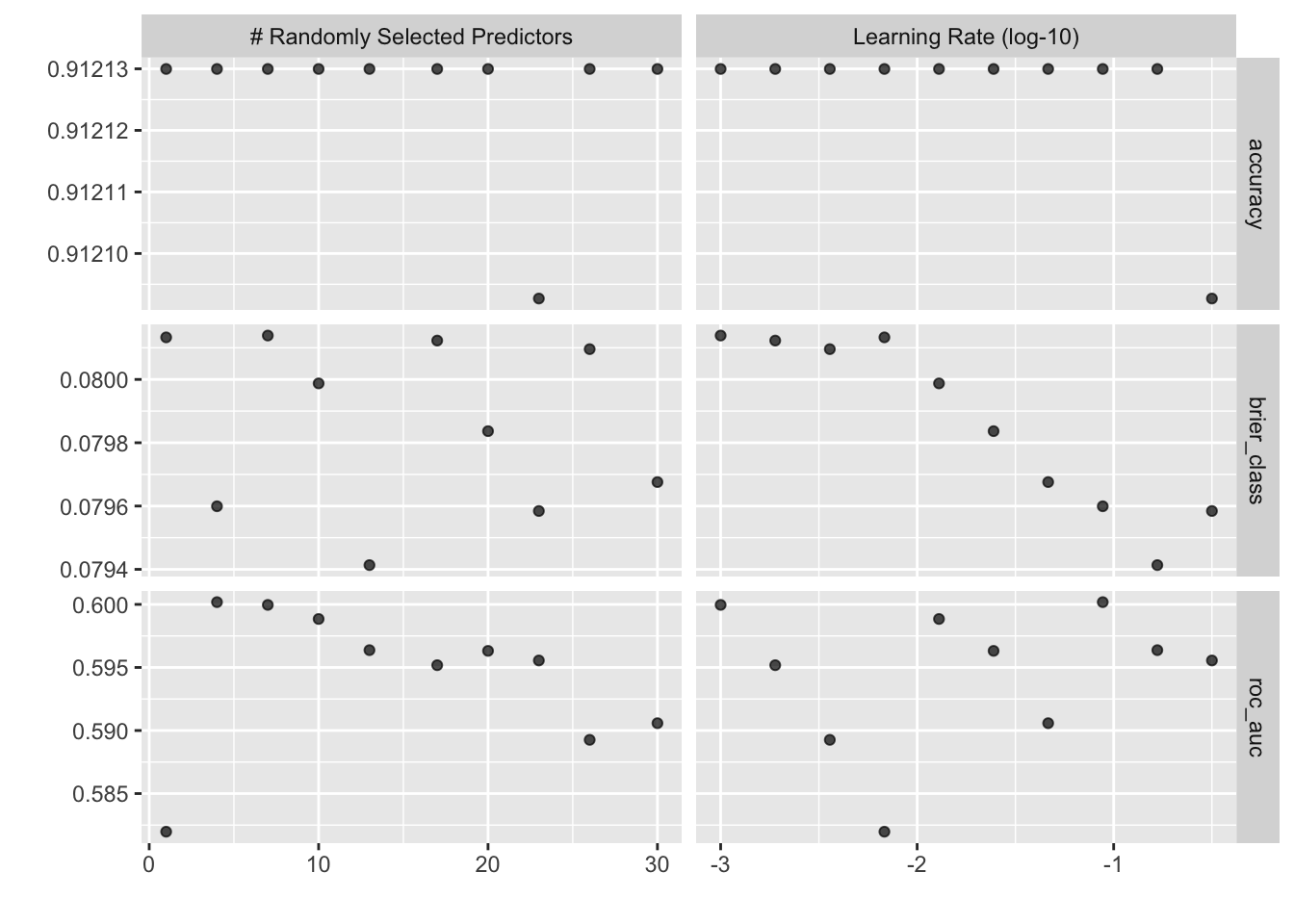

Comparing results

The steps in this section should not be part of an every day workflow. It is included here for comparison purposes. We are comparing the results from Spark versus local R.

results <- tune_grid(spec_bt, recipe_basic, readmission_folds)
#> i Creating pre-processing data to finalize 1 unknown parameter: "mtry"

# Use show_best() to compare the recommendations
show_best(results, metric = "roc_auc")
#> # A tibble: 5 × 8
#>    mtry learn_rate .metric .estimator  mean     n std_err .config         
#>   <int>      <dbl> <chr>   <chr>      <dbl> <int>   <dbl> <chr>           
#> 1     4     0.0880 roc_auc binary     0.600    10 0.00425 pre0_mod02_post0
#> 2     7     0.001  roc_auc binary     0.600    10 0.00434 pre0_mod03_post0
#> 3    10     0.0129 roc_auc binary     0.599    10 0.00467 pre0_mod04_post0
#> 4    13     0.167  roc_auc binary     0.596    10 0.00391 pre0_mod05_post0
#> 5    20     0.0245 roc_auc binary     0.596    10 0.00509 pre0_mod07_post0

show_best(spark_results, metric = "roc_auc")
#> # A tibble: 5 × 8
#>    mtry learn_rate .metric .estimator  mean     n std_err .config         
#>   <int>      <dbl> <chr>   <chr>      <dbl> <int>   <dbl> <chr>           
#> 1     4    0.0880  roc_auc binary     0.600    10 0.00425 pre0_mod02_post0
#> 2     7    0.00100 roc_auc binary     0.600    10 0.00434 pre0_mod03_post0
#> 3    10    0.0129  roc_auc binary     0.599    10 0.00467 pre0_mod04_post0
#> 4    13    0.167   roc_auc binary     0.596    10 0.00391 pre0_mod05_post0
#> 5    20    0.0245  roc_auc binary     0.596    10 0.00509 pre0_mod07_post0

The results are identical because Spark is running locally. It should not be surprising if the results are different if using Spark remotely. Differences in Operating System, R run-time, and R packages can affect the results. Reproducibility is not impacted because the remote job will always return the same results. sparklyr replicates how tidymodels reliably sets the seed during the tuning.

Parallel processing in Spark

In Spark, the term job differs from the term task. A single job contains multiple tasks that can run in parallel. Spark will run as many concurrent tasks as there are CPU cores that the cluster makes available to that particular job. In the example on Figure 3, a single job is running 4 tasks in parallel thanks to each running in a separate core.

flowchart RL
  subgraph j [<b>Job</b>]
   t1[<b>Task 1</b> <br/> Core 1]
   t2[<b>Task 2</b> <br/> Core 2]
   t3[<b>Task 3</b> <br/> Core 3]
   t4[<b>Task 4</b> <br/> Core 4]
  end
  style j fill:#F8DDBF,stroke:#666,color:#000;
  style t1 fill:#F7EADC,stroke:#666,color:#444;
  style t2 fill:#F7EADC,stroke:#666,color:#444;
  style t3 fill:#F7EADC,stroke:#666,color:#444;
  style t4 fill:#F7EADC,stroke:#666,color:#444;
  linkStyle default stroke:#666,color:#000

Figure 3: Job vs. Task in Spark example

Spark parallelism impacts tune_grid_spark() in one of two ways. The way is determined by how parallel_over is set in its control grid:

spark_results <- tune_grid_spark(
  sc = sc,
  object = spec_bt,
  preprocessor = recipe_basic, 
  resamples = readmission_folds,
  # Pass a `control_grid()` object to `control`
  control = control_grid(parallel_over = "resamples") 
  )

sparklyr accepts the two values that tune accepts for parallel_over. This is how each will behave in Spark:

resamples (default) - The tuning is performed in parallel over the resamples alone. In the example, readmission_folds has 10 folds/resamples. If we had 4 tasks available from Spark, then the 10 folds would be distributed across that number of tasks. This means that some two tasks will run 2 folds, the other two will run 3 folds, see Figure 4. Inside the tasks, the 2 or 3 folds will run sequentially, but the 4 tasks will start processing folds at the same time.

flowchart RL
  subgraph j [<b>Job</b>]
   t1[<b>Task 1</b> <br/> Fold 1 <br/> Fold 2 <br/> Fold 3]
   t2[<b>Task 2</b> <br/> Fold 4 <br/> Fold 5 <br/> Fold 6]
   t3[<b>Task 3</b> <br/> Fold 7 <br/> Fold 8]
   t4[<b>Task 4</b> <br/> Fold 9 <br/> Fold 10]
  end
  style j fill:#F8DDBF,stroke:#666,color:#000;
  style t1 fill:#F7EADC,stroke:#666,color:#444;
  style t2 fill:#F7EADC,stroke:#666,color:#444;
  style t3 fill:#F7EADC,stroke:#666,color:#444;
  style t4 fill:#F7EADC,stroke:#666,color:#444;
  linkStyle default stroke:#666,color:#000

Figure 4: How “resamples” works in Spark

everything - The tuning will be performed in parallel for each combination of resamples and tuning parameters In the example, we used the default for the grid argument, which is 10. That indicates the number of candidate parameter sets to be created automatically. The 10 parameter sets, are then combined with the 10 folds/resamples, giving us 100 total combinations. If we had 4 tasks available from Spark, then each will run 25 combinations.

flowchart RL
  subgraph j [<b>Job</b>]
   t1[<b>Task 1</b> <br/> Fold 1 - Combo 1 <br/> ... <br/> ...  <br/> Fold 3 - Combo 5]
   t2[<b>Task 2</b> <br/> Fold 3 - Combo 6 <br/> ... <br/> ...  <br/> Fold 5 - Combo 10]
   t3[<b>Task 3</b> <br/> Fold 6 - Combo 1 <br/> ... <br/> ...  <br/> Fold 8 - Combo 5]
   t4[<b>Task 4</b> <br/> Fold 8 - Combo 6 <br/> ... <br/> ...  <br/> Fold 10 - Combo 10]
  end
  style j fill:#F8DDBF,stroke:#666,color:#000;
  style t1 fill:#F7EADC,stroke:#666,color:#444;
  style t2 fill:#F7EADC,stroke:#666,color:#444;
  style t3 fill:#F7EADC,stroke:#666,color:#444;
  style t4 fill:#F7EADC,stroke:#666,color:#444;
  linkStyle default stroke:#666,color:#000

Figure 5: How “everything” works in Spark

Despite the number of resamples, or number of tuning + resamples combinations, the limit of how many processes run in parallel is set by how many tasks are created for the job. The more nodes and cores there are available in the Spark cluster, the more possible parallel tasks could be scheduled to run for the job.

Retrieving predictions a.k.a `save_pred = TRUE`

sparklyr supports getting the out-of-sample predictions if they are saved. That is done by using control_grid() when calling tune_grid_spark().

spark_results <- tune_grid_spark(
  sc = sc,
  object = spec_bt,
  preprocessor = recipe_basic, 
  resamples = readmission_folds,
  control = control_grid(save_pred = TRUE)
  )
#> i Creating pre-processing data to finalize 1 unknown parameter: "mtry"

Spark will execute an additional small job. The job simply reads the files that have the predictions created during the tuning job. The data from the files is incorporated to the tune results object that sparklyr returns.

collect_predictions(spark_results)
#> # A tibble: 536,360 × 9
#>    .pred_class .pred_Yes .pred_No id     readmitted  .row  mtry learn_rate
#>    <chr>           <dbl>    <dbl> <chr>  <chr>      <int> <int>      <dbl>
#>  1 No             0.0882    0.912 Fold01 No            10     1    0.00681
#>  2 No             0.0889    0.911 Fold01 Yes           31     1    0.00681
#>  3 No             0.0883    0.912 Fold01 No            51     1    0.00681
#>  4 No             0.0879    0.912 Fold01 No            52     1    0.00681
#>  5 No             0.0889    0.911 Fold01 No            62     1    0.00681
#>  6 No             0.0879    0.912 Fold01 No            89     1    0.00681
#>  7 No             0.0884    0.912 Fold01 Yes          102     1    0.00681
#>  8 No             0.0878    0.912 Fold01 No           112     1    0.00681
#>  9 No             0.0881    0.912 Fold01 No           146     1    0.00681
#> 10 No             0.0879    0.912 Fold01 No           150     1    0.00681
#> # ℹ 536,350 more rows
#> # ℹ 1 more variable: .config <chr>

Verbosity

tune_grid_spark() also supports a more verbose output during tuning. But unlike the function in tune, sparklyr focuses more on stages and timings of each stage. It does not report on individual iterations as tune does.

spark_results <- tune_grid_spark(
  sc = sc,
  object = spec_bt,
  preprocessor = recipe_basic, 
  resamples = readmission_folds,
  control = control_grid(verbose = TRUE)
  )
#> i Creating pre-processing data to finalize 1 unknown parameter: "mtry"
#> ℹ Uploading model, pre-processor, and other info to the Spark session
#> ✔ Uploading model, pre-processor, and other info to the Spark session [147ms]
#> 
#> ℹ Uploading the re-samples to the Spark session
#> ✔ Uploading the re-samples to the Spark session [8ms]
#> 
#> ℹ Copying the grid to the Spark session
#> ✔ Copying the grid to the Spark session [7ms]
#> 
#> ℹ Executing the model tuning in Spark
#> ✔ Executing the model tuning in Spark [4.3s]
#>

Conclusion

The two goals of this approach is to shorten the time it takes to tune the model, and to do this without re-writing the code so that it can run in Spark. The disadvantage is that the data has to be uploaded to Spark. This means that there are size constraints for the data itself. Again, the focus is not so much “big data”, but to accelerate tuning by taking advantage of using the distributed computing in Spark. If you need to tune models that use very large amounts of data, then consider using Spark ML directly.